Rolling rankings
Lowest-RMSE sets change frequently
In 12-month rolling evaluations, winner-set switch rates range from 17.9% to 38.5% across target-horizon combinations, with a mean switch rate of 29.1%.
Lower average forecast error does not by itself establish a statistically distinguishable or persistent advantage. This study evaluates average accuracy, statistical distinguishability, and temporal stability separately within a common data-rich macroeconomic forecasting design.
The analysis uses the June 2026 FRED-MD vintage and evaluates twelve forecasting approaches across CPI inflation, PCE inflation, industrial production growth, and the monthly change in the unemployment rate at 1-, 3-, 6-, and 12-month horizons. The comparison includes nine individual models and three forecast combinations. The central question is how much confidence can be placed in the observed average rankings once formal inference and temporal diagnostics are considered.
Four headline statistics summarize how average ranking, formal inference, and temporal stability provide different assessments in the reported pseudo-out-of-sample exercise.
Three paper-aligned exhibits show average RMSE ranking, numerical rank versus MCS survival, and the temporal concentration of loss differences. Click any figure to inspect the full-resolution image.
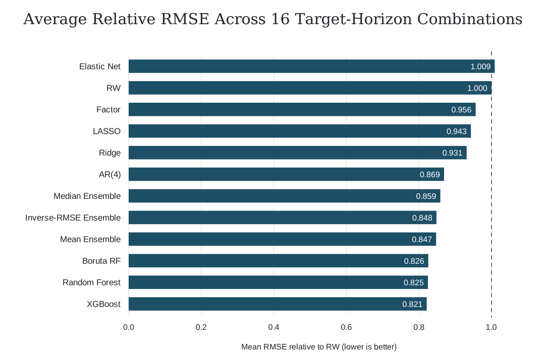
Average relative RMSE varies across the twelve approaches. XGBoost is lowest at 0.821, and the dashed line marks equality with RW. The ranking is numerical and does not by itself establish statistical separation.
Open full-size figure ↗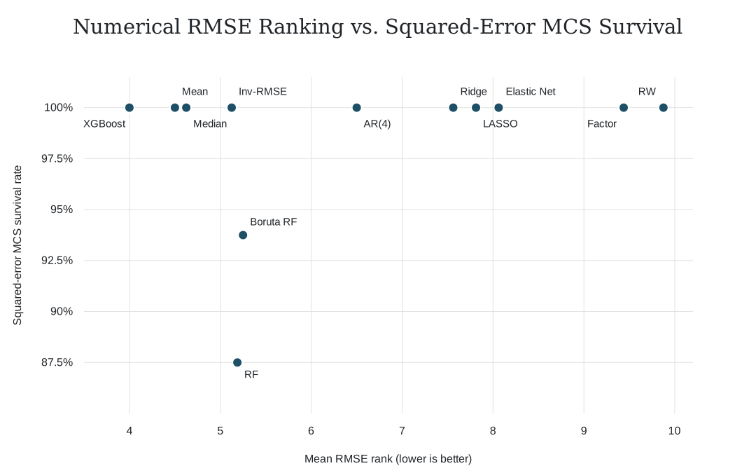
Mean RMSE ranks differ, while most approaches survive every squared-error Model Confidence Set panel. MCS survival does not prove equal accuracy; it reflects limited evidence for eliminating candidates.
Open full-size figure ↗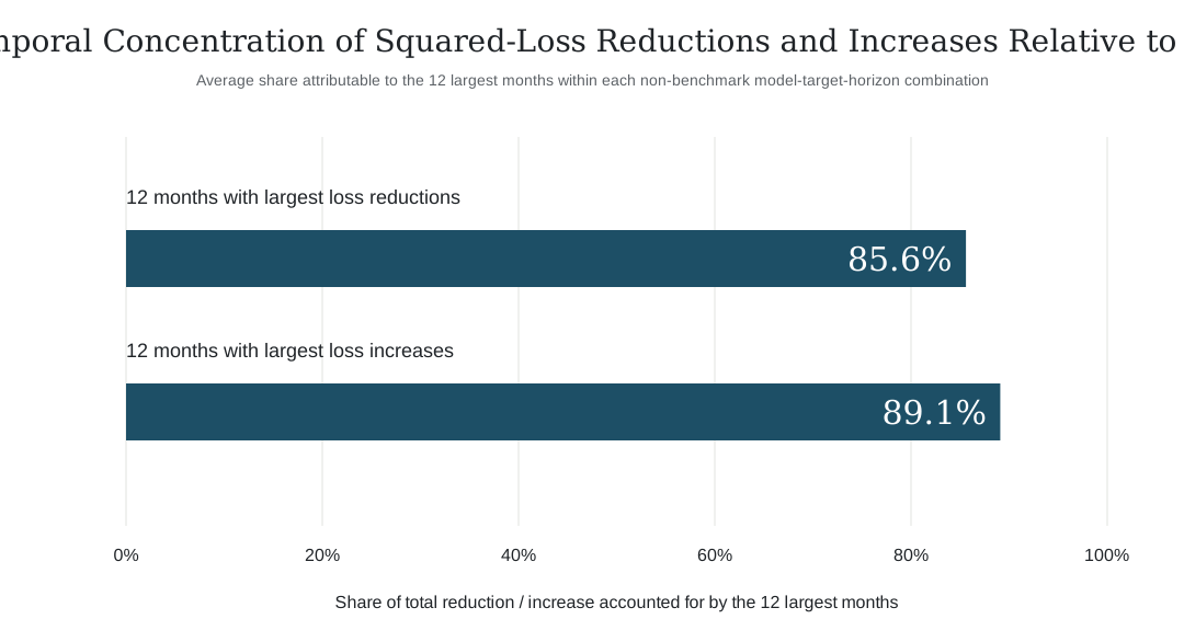
For squared loss, the twelve months with the largest reductions relative to RW account, on average, for 85.6% of total loss reduction, while the twelve months with the largest increases account for 89.1% of total loss increase.
Open full-size figure ↗Four U.S. monthly targets are evaluated with the June 2026 FRED-MD vintage under common predictor screening, lagging, and missing-data rules.
Direct forecasts use 360-month rolling estimation windows and up to 90 target months from December 2018 through May 2026, before target-specific exclusions.
Nine individual models span persistence, autoregression, regularized linear models, PCA factors, and tree learners; mean, median, and inverse-RMSE combinations are added.
Average RMSE rankings show clearer numerical differences than formal inference suggests.
XGBoost's average relative RMSE of 0.821 corresponds to a 17.9% average reduction relative to the persistence benchmark across the sixteen target-horizon combinations.
None of the 176 squared-error Diebold-Mariano comparisons rejects equal predictive accuracy in favor of an alternative after Holm adjustment. Five absolute-error comparisons reject, all at one-month industrial production.
From a multi-model perspective, the 90% Model Confidence Set retains all twelve approaches in 25 of 32 panels, and no panel retains fewer than ten. Survival does not prove equal accuracy; the available loss data provide limited evidence for eliminating most candidates at the chosen confidence level.
The set of lowest-RMSE models changes frequently across rolling windows, and loss differences are highly concentrated in a small number of dates.
In 12-month rolling evaluations, winner-set switch rates range from 17.9% to 38.5% across target-horizon combinations, with a mean switch rate of 29.1%.
Removing only the date with the largest RW squared error within each target-horizon combination raises the best average relative RMSE from 0.821 to 0.916. After twelve such exclusions, RW leads on average.
Historical values come from one revised June 2026 FRED-MD vintage. The exercise does not reconstruct real-time data vintages, release lags, or historical revisions.
The primary evaluation contains at most 90 target months and includes the COVID-19 collapse and reopening, limiting statistical power and the range of macroeconomic environments represented in the sample.
The conclusions apply to the stated linear, factor, tree-based, and combination methods. Neural networks and time-series foundation models are outside this model set.
Rolling winner-set changes and loss concentration are descriptive diagnostics. They complement formal inference but are not formal instability or state-dependence tests.
These companion articles explain methods used directly in the study or needed to interpret its design and evidence.
Explains the information boundary behind the paper's repeated pseudo-out-of-sample evaluation.
Clarifies the fixed-length rolling estimation window used in the paper and the trade-off that window choice creates.
Explains how timing, data construction, and model-development choices can let future information enter a historical forecasting exercise.
Explains the pairwise loss-differential test used to assess whether forecast-accuracy differences are statistically distinguishable.
Explains the set-valued comparison used when the available loss data do not sharply separate many forecasting approaches.
The public replication repository contains forecasting and statistical-analysis code, versioned outputs, table and figure data exports, the locked R environment, data-acquisition guidance, and release validation tools. The source FRED-MD CSV is not redistributed.
Research code, reproducibility documentation, versioned outputs, and paper exports.
Open GitHub ↗Latest tagged public package: v1.0.0. Versioned software and replication snapshot for the reported research design and outputs.
Open release ↗The interactive forecasting dashboard lets readers explore model performance and related forecasting evidence. It complements the versioned paper and replication materials; it does not replace the paper's fixed empirical record.